BigQuery Graph Series | Part 2: (Tutorial) Build a BigQuery Graph from unstructured data

BigQuery Graph Series | Part 2: (Tutorial) Build a Graph from unstructured data

In Part 1, we explored how to unlock unstructured “dark data” by using a Hybrid AI approach — pairing Document AI’s parsing precision with Gemini’s reasoning — to build a structured knowledge graph natively in BigQuery.

Now it’s time to get hands on! Welcome to part 2 of this series:

Part 1: From Dark Data to Knowledge Graphs

Part 2 (this post): Tutorial: Build a BigQuery Graph from unstructured data

Part 3: Query and visualize your BigQuery Graph

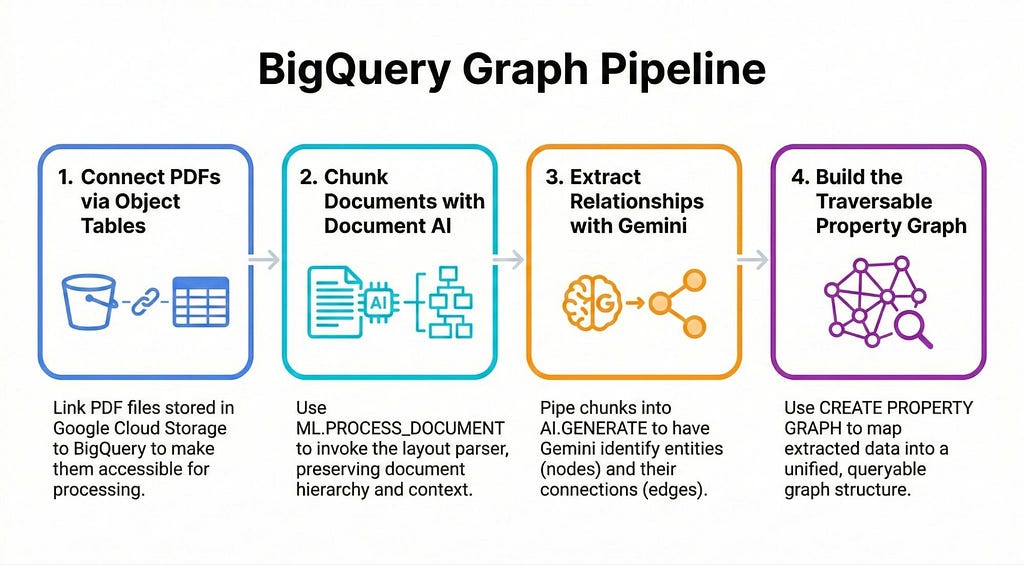
In this post, we’ll walk through a simple, practical example to turn your unstructured data in Google Cloud Storage into a living, traversable graph using only BigQuery:

Tutorial: Build a BigQuery Graph from unstructured data

Imagine you have thousands of PDFs containing vital information about products and parts. Details such as product parts, materials and related error codes are scattered across all the documents. We need to connect these dots to answer business-critical questions such as:

“Which customers purchased products that contain ‘Fiberglass’?” — this is a complex query that requires hopping from customer purchases, to products to parts and finally to Material.

There are a few ways you can build this out, I’ve opted for a simple approach that shows all the components you’ll need to have in place. This should serve as a baseline that you can build upon for your use case.

💡 Want the full code? This tutorial provides a high-level overview with simplified SQL snippets to explain the core concepts. Checkout this notebook for the complete, runnable code.

Getting Started

💡 Heads up: Your project must be allowlisted to use the BigQuery Graph feature (currently in private preview).

Before you dive in, you’ll need to make sure your Google Cloud project has all the relevant APIs enabled (like BigQuery, and Vertex AI and Document AI).

Step 1: Create an Object Table

Assuming you have your unstructured PDF manuals stored in a Google Cloud Storage (GCS) bucket, our first step is to make those files visible to BigQuery using an Object Table.

CREATE OR REPLACE EXTERNAL TABLE `my_project.my_dataset.document_object_table`
WITH CONNECTION `us.vertex-conn`
OPTIONS(
 object_metadata = 'SIMPLE',
 uris = ['gs://my-bucket/demo_docs/*.pdf']

Step 2: Create a connection to the Document AI Layout Parser

You’ll then need to create a Doc AI Processor of type Layout Parser. You can do this in the console, or programmatically via the notebook:

Once that’s set up in the Cloud Console, we create a remote model in BigQuery to connect to this processor:

CREATE OR REPLACE MODEL `my_dataset.docai_model`
REMOTE WITH CONNECTION DEFAULT
OPTIONS (
  REMOTE_SERVICE_TYPE = 'CLOUD_AI_DOCUMENT_V1',
  DOCUMENT_PROCESSOR = 'your_processor_id'
);

Step 3: Parse with Document AI

Next, we use the ML.PROCESS_DOCUMENT function to call the Document AI Layout Parser and flatten the results into a readable table.

⚠️ Gotcha: ML.PROCESS_DOCUMENT has a limit of 130 pages per document and a 120-second timeout. If your manuals are larger, you may need to split them in GCS before processing or use an asynchronous batch processing pipeline outside of BigQuery for those specific files.

CREATE OR REPLACE TABLE `my_dataset.processed_documents` AS
SELECT * FROM ML.PROCESS_DOCUMENT(
  MODEL `my_dataset.docai_model`,
  TABLE `my_dataset.document_object_table`
);

💡 Note: Document AI returns a nested JSON object. In the companion notebook, we use standard BigQuery JSON functions to flatten this into clean text chunks before passing it to Gemini.

Step 4: Extracting with Gemini 3.1 Pro

Here is where the real magic happens. We use BigQuery’s AI.GENERATE function to invoke Gemini. We’ll use Gemini 3.1 Pro, but you can specify any generally available or preview model.

We instruct Gemini to act as a “Technical Knowledge Graph Extractor” and output a structured JSON array of relationships.

CREATE OR REPLACE TABLE `my_dataset.extracted_knowledge_graph` AS
SELECT
  uri, r.*
FROM (
  SELECT AI.GENERATE(
      -- We pass the prompt and the document content together
      """          
      You are an expert technical knowledge graph extractor.
      
      TASK:
      Extract a comprehensive list of ALL component relationships from the provided text.
      
      VALID ENTITY TYPES:
      - Product
      - Part
      - Material
      - Other
      
      ALLOWED RELATIONSHIP TYPES:
      - CONTAINS_PART: (Product) -> (Part ID)
      - MADE_OF: (Part ID) -> (Material Name)
      - CONNECTS_TO: (Part A) -> (Part B)
      """ || content,
      
      output_schema => """
        relationships ARRAY<STRUCT<
          subject STRING, subject_entity_type STRING,
          relationship STRING,
          object STRING, object_entity_type STRING,
        >>
      """,
      endpoint => 'https://aiplatform.googleapis.com/v1/projects/your-project-id/locations/global/publishers/google/models/gemini-3.1-pro-preview'
    ) AS extracted_data
  FROM `my_dataset.processed_documents`
), UNNEST(extracted_data.relationships) AS r;

💡Nobody like parsing LLM outputs. We use the output_schema argument to enforce a strict JSON structure, making our pipeline more deterministic and robust.

Step 5: Creating Node and Edge Tables

So we’ve created a flattened table where every row represents a single relationship: Subject -> Relationship -> Object.

To turn this into a graph, BigQuery needs us to organize this raw output into tables representing our distinct entities (Nodes) and the connections between them (Edges). We do this by slicing that extracted table based on the relationship types.

💡 Note: You can do this part programmatically, but I’m sticking simple SQL statements so you can easily see the underlying data structure needed to build the graph.

Creating Node Tables (The Entities): We extract unique entities by filtering the relationships. For example, everything that is the “object” of a “MADE_OF” relationship becomes a Material node.

CREATE OR REPLACE TABLE `my_dataset.part_nodes`
AS
SELECT DISTINCT subject AS part_name
FROM `my_dataset.extracted_knowledge_graph`
WHERE subject_entity_type = 'Part';

Creating Edge tables (The relationships): To connect parts to their materials, we select the “subject” (the part) and the “object” (the material) wherever the relationship is “MADE_OF”.

CREATE OR REPLACE TABLE `my_dataset.edges_part_material`
AS
SELECT subject AS part_name, object AS material_name
FROM `my_dataset.extracted_knowledge_graph`
WHERE relationship = 'MADE_OF';

Step 6: The Grand Finale — CREATE PROPERTY GRAPH

And finally, the feature that ties it all together. BigQuery’s CREATE PROPERTY GRAPH DDL allows us to map tables into a single logical graph entity:

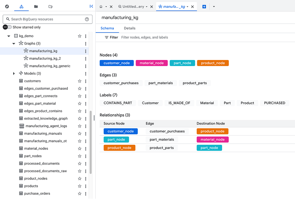
CREATE OR REPLACE PROPERTY GRAPH `my_dataset.manufacturing_kg`
  NODE TABLES (
    `my_dataset.customers` AS customer_node KEY (customer_id) LABEL Customer,
     `my_dataset.products` AS product_node KEY (product_name) LABEL Product,
    `my_dataset.part_nodes` AS part_node KEY (part_name) LABEL Part,
    `my_dataset.material_nodes` AS material_node KEY (material_name) LABEL Material
  )
  EDGE TABLES (
    `my_dataset.edges_product_contains` AS product_parts
      SOURCE KEY (product_name) REFERENCES product_node
      DESTINATION KEY (part_name) REFERENCES part_node
      LABEL CONTAINS_PART,
      
    `my_dataset.edges_part_material` AS part_materials
      SOURCE KEY (part_name) REFERENCES part_node
      DESTINATION KEY (material_name) REFERENCES material_node
      LABEL IS_MADE_OF
  );

🌟 A major advantage of doing this in BigQuery is that this Graph can serve as a bridge your structured and unstructured data. You can include existing relational tables — like your customers or products tables — alongside your newly extracted part_nodes and material_nodes. This allows you to connect your unstructured “dark data” directly to your core business data.

Breaking Down the Syntax:

Node Tables: Defines which BigQuery tables act as your core entities. Assigning a LABEL (e.g., Product) categorizes these nodes, allowing you to easily query them later using syntax like MATCH (n:Product).
Edge Tables: These define the relationships between your nodes. By assigning a LABEL (like CONTAINS_PART), you categorize the type of connection, allowing you to filter by specific relationship types when querying the graph.
The Stitching Logic: The SOURCE KEY and DESTINATION KEY define the exact direction and topology of your graph. They explicitly map the columns in your edge table directly to the primary keys of your node tables .

💡 Moving Forward: You can (and will likely want to) also include vector embeddings as properties on your nodes to enable “Hybrid Search” (finding a node conceptually and then validating it structurally), but we won’t cover that pattern in this specific post.

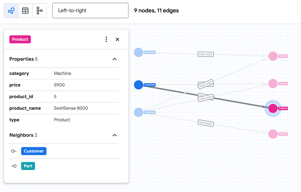
We have our BigQuery Graph!

Phew! We haven’t just created a bunch of tables; we’ve built an ontology. We now have the ability to traverse an enterprise-wide map built from “dark data,” allowing us to run elegant Graph Queries (GQL) that do away with complex and costly JOIN statements.

Continue on to part 3 to see how you can visualize and query this Graph!

Keep Reading!

BigQuery Graph Notebook
BigQuery Object Tables
ML.PROCESS_DOCUMENT Function
ML.GENERATE_TEXT Documentation

BigQuery Graph Series | Part 2: (Tutorial) Build a BigQuery Graph from unstructured data was originally published in Google Cloud – Community on Medium, where people are continuing the conversation by highlighting and responding to this story.

Source Credit: https://medium.com/google-cloud/bigquery-graph-series-6a768ccb351b?source=rss—-e52cf94d98af—4