
Key Insights:
- The static threshold fallacy: Deploying a single, hardcoded cosine similarity threshold across diverse queries in high-dimensional spaces is mathematically brittle; score distributions shift drastically depending on the query’s semantic density.
- The cost of precision: While comprehensively training a specialized thresholding model yields the highest accuracy, BigQuery’s on-demand scan costs and high compute latencies can make exhaustive scanning unfeasible for some production use cases.
- The multimodal complexity: Google’s Gemini Embeddings 2 operates in a shared, natively multimodal 3072-dimensional space, introducing “modality gaps” where cross-modal similarities operate within highly compressed numerical bands.
- Algorithmic workarounds: Density-weighted sampling and annular synthetic probing present two innovative methodologies to dynamically approximate optimal thresholds, yet possess unique underlying assumptions that must be carefully considered.
Determining the exact boundary where a retrieved vector transitions from “relevant” to “irrelevant” is one of the most notoriously difficult challenges in modern information retrieval. When dealing with massive datasets housing millions of unstructured assets, calculating the perfect cosine similarity threshold is often treated as an afterthought — a static configuration variable guessed after eyeballing a few search results. The optimal solution is, without debate, to train a dedicated ranking model or rigorously test against a meticulously labeled dataset of millions of examples to discover the precise threshold. However, in the real world of limited budgets, rapid iteration cycles, and continually evolving data manifolds, full-scale training is frequently unfeasible.
This report delves deeply into the mechanics of cosine similarity thresholding, specifically tailored for Google’s Gemini Embeddings 2 architecture [1]. We will explore the geometric realities of high-dimensional vector spaces, analyze the inherent complexities of multimodal embeddings, and critically dissect algorithmic strategies to dynamically approximate optimal thresholds when exhaustive testing is off the table.
Executive Summary
Determining an optimal, dynamic cosine similarity threshold is critical for precision, but computationally expensive to execute in real-time. In this post, we evaluate two programmatic methodologies to find this boundary without exhaustive model training.
Method 1 (Density-Weighted Sampling) is statistically rigorous, focusing evaluation budgets entirely on the decision boundary. However, it is prohibitively expensive to run in production, as full dataset distance scans incur exorbitant BigQuery compute costs.
Method 2 (Annular Probing) is geometrically elegant, using synthetic vectors to quickly map out the outer boundaries of a query’s neighborhood via fast index searches. Unfortunately, it fails against the mathematical reality of high dimensions, as synthetic probes frequently land in empty space and trigger index quantization errors.
Ultimately, neither approach works perfectly in isolation. The recommended strategy is a hybrid approach: combine methodologies and utilize ScaNN-based nearest neighbors (such as Vertex AI Vector Search) whenever an exhaustive search is unnecessary.
The Architectural Context of Gemini Embeddings 2
Before critiquing specific thresholding algorithms, it is critical to understand the environment in which these thresholds operate. Gemini Embeddings 2 is not merely a textual encoder; it is a natively multimodal foundational model [1].
A Unified Vector Space
Gemini Embeddings 2 maps text, images, video (up to 120 seconds), audio (up to 80 seconds), and complex documents (like PDFs) into a single, unified semantic space [1, 2]. This unified representation means that a query comprising an English sentence can be directly compared against a photograph using simple cosine similarity [1,2].
In this architecture, vectors are instantiated by default in 3072 dimensions [1]. The model employs Matryoshka Representation Learning (MRL), a structural technique that allows developers to truncate these vectors down to smaller dimensions — such as 1536, 768 — without requiring any retraining [1]. The most semantically critical information is front-loaded into the earliest dimensions.
The Modality Gap and Compressed Similarity Ranges
A crucial phenomenon to understand when thresholding Gemini Embeddings 2 is the “modality gap”. While images and text share the same vector space, they naturally tend to cluster in slightly different hyper-dimensional neighborhoods [3]. To the model, a photograph of a dog and the text “a photograph of a dog” are conceptually identical but structurally distinct.
As a result, cross-modal similarity scores are heavily compressed. When searching across modalities, similarity scores rarely reach the 0.8 or 0.9 ranges seen in pure text-to-text semantic matches. Instead, they typically operate in a compressed band between 0.15 and 0.55 [3]. Within this seemingly narrow window, the semantic signal is remarkably strong. A score of 0.5 represents a very high match, while anything below 0.22 indicates little to no match [3].
This compression dictates that any thresholding strategy must be highly sensitive. A shift of 0.1 in a threshold might seem mathematically insignificant, but in a compressed cross-modal space, it can represent the difference between high-precision retrieval and catastrophic false-positive noise.
The Fallacy of Static Thresholding
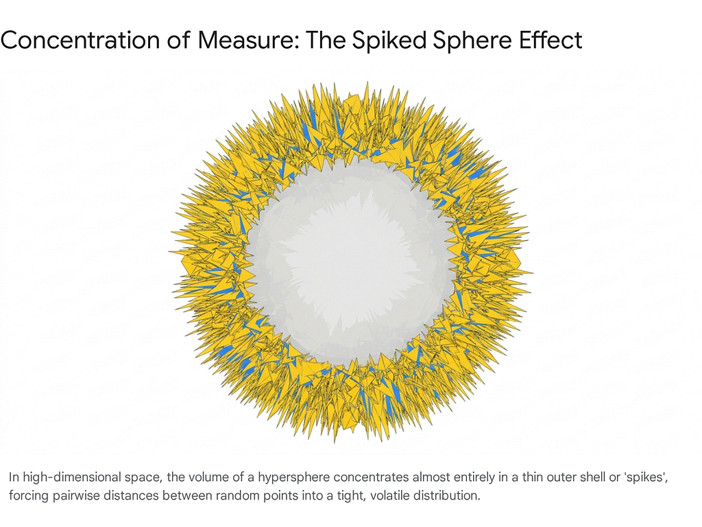
The fundamental problem with vector databases is that distance distributions are query-dependent. If you query a database for a highly generic concept, such as “vehicles,” the resulting vector neighborhood will be densely packed. The nearest neighbors might have cosine similarities of 0.85, and the 10,000th neighbor might still have a similarity of 0.75. Conversely, if you query for a highly specific or out-of-domain concept, such as “18th-century left-handed surgical instruments,” the closest match in the database might only yield a cosine similarity of 0.40.
If a system relies on a static threshold of 0.70, the first query will return 10,000 results (many of which may be irrelevant edge cases), while the second query will return absolutely nothing, despite the database potentially containing a somewhat relevant 19th-century right-handed instrument at a 0.65 similarity. Dynamic thresholding — adjusting the boundary based on the specific topology of the query’s neighborhood — is therefore essential for maintaining a precision.
Below, we critically evaluate two such methodologies.
Critique of Method 1: Density-Weighted Sampling Strategy
The first proposed methodology attempts to find a threshold by sampling real data from the database, weighing those samples around a historically informed “anchor” point, labeling a small batch using a Gemini, and applying rigorous statistical confidence intervals to guarantee precision.
Method Breakdown and Geometric Logic
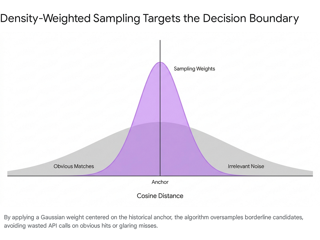
Setup: Establishing the Prior: The method begins by establishing an `anchor`, representing a historical average threshold. It then refines this prior by pulling the retrieval tail — authentic low-ranked hits (hard negatives) from a `vector_search` — and averaging their distances to calibrate the boundary.
Meat: Density-Weighted Sampling and Wilson Intervals: Once the anchor is set, the system performs a distance scan across the dataset (using BigQuery or a `TABLESAMPLE` equivalent). It applies a Gaussian weight centered on the anchor:
weights = np.exp(-((distances — anchor)**2) / (2 * sigma**2))
This ensures that the samples selected for Gemini to grade are heavily concentrated near the suspected decision boundary, rather than wasting labeling budget on obvious true positives (score > 0.8) or obvious true negatives (score < 0.1).
The samples are graded via a batched call. Finally, the system calculates the cumulative precision for candidate thresholds. It uses the standard Wilson score interval to measure statistical uncertainty.
Definition & Analogy: The Wilson score interval is an advanced formula for calculating statistical confidence that elegantly handles extreme probabilities and small sample sizes. Think of it like trying to estimate a baseball player’s true batting average after they have only had 5 at-bats. If they hit 5 out of 5, a naive calculation says they are a 100% perfect hitter. The Wilson interval effectively adds “dummy” average at-bats to the calculation, assuming the player is average until statistically proven otherwise.
Relevance: Traditional normal approximation intervals (like the Wald interval) fail catastrophically when proportions are near 0 or 1, or when sample sizes are extremely small. The Wilson interval provides asymmetric, reliable confidence bounds, ensuring the system does not prematurely accept a weak threshold simply because a tiny sample happened to get lucky during Gemini grading.
If the confidence interval (CI) is too wide (exceeding a 10% uncertainty SLA), the system iterates: it shifts the anchor to the new candidate boundary, tightens the Gaussian variance, and samples again.
Synthesis: Pros and Cons of Method 1 —
Pros:
1. Budget Efficiency through Boundary Focus: Machine learning classifiers gain the most information from boundary cases (support vectors). By focusing the sampling budget specifically around the suspected threshold via Gaussian weights, this method avoids wasting API calls on unambiguous matches.
2. Statistical Rigor: The integration of the Wilson score interval is highly commendable, providing mathematical safeguards against sparse, lucky sampling bounds.
3. Real-Data Grounding: Because this method samples directly from the actual database (e.g., via BigQuery `VECTOR_SEARCH`), it naturally accounts for the true underlying data manifold.
Cons:
1. The BigQuery Distance Scan Cost: BigQuery charges based on the columns and partitions your query touches, not the result size. Therefore, a full distance scan across a multi-million row table could cost a few $s, for use cases where many users interact this could be prohibitive. .
2. Vulnerability to the Modality Gap: As established, Gemini Embeddings 2 operates in a compressed 0.15 to 0.55 range for cross-modal tasks [3]. A Gaussian `sigma` value must be extraordinarily tight to be useful in this compressed space. If `sigma` is too wide, the sampling will degenerate into uniform random sampling across the narrow active band.
Critique of Method 2: Annular Probing (ScaNN Ring-Fencing)
The second proposed methodology takes a radically different, highly geometric approach. Instead of sampling existing data to find the threshold, it generates synthetic vector “probes” at specific mathematical distances (rings) from the query, queries the vector index to see what real data lives near those probes, and searches for the “precision cliff.”
Method Breakdown and Geometric Logic
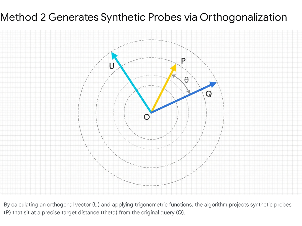
Setup: Synthetic Orthogonal Probes and Gram-Schmidt
This method defines a set of coarse distance rings (e.g., `D = [0.15, 0.20, … 0.40]`). For a normalized unit vector Q, the cosine distance translates directly to an angle =(1-D).
To create a probe at exactly distance D, the method generates a random Gaussian vector n, removes its component along Q using the **Gram-Schmidt process** to create an orthogonal vector U, and then combines them:
P = Q * np.cos(theta) + U * np.sin(theta)
Definition & Analogy: The Gram-Schmidt process is a mathematical method for taking a set of vectors and turning them into a strictly perpendicular (orthogonal) set. Imagine a flagpole standing on the ground, casting a shadow as the sun moves. The sun’s rays and the ground are mixed vectors. Gram-Schmidt is the geometric equivalent of finding the exact, perfect 90-degree ‘shadow’ of a line, ensuring total independence.
Relevance: In this algorithm, it ensures that the synthetic probe vector strictly explores outward distance perpendicular to the query, rather than accidentally drifting closer or overlapping with the query’s direct semantic path.
Meat: ScaNN Retrieval and Ring-Fencing
These synthetic probes are fed into Google’s Scalable Nearest Neighbors (ScaNN) algorithm [4]. Because ScaNN is optimized for Approximate Nearest Neighbor (ANN) search, it returns results in milliseconds (often <10ms for a 1M vector index).
However, ScaNN returns the neighbors closest to the *probe*. Some of these neighbors might actually be very close to the original query Q (falling inward), while others might be further away. To fix this, the method filters the ScaNN results to keep only the “crust” — assets whose actual distance to Q sits within a tight tolerance (`RING_TOL`) of the target distance D.
These surviving assets are sampled, graded by Gemini, and used to calculate the precision at that specific ring. The system finds the largest distance ring that still passes the 90% Precision SLA, and then performs a binary search (bisection) to refine the threshold to a micro-resolution of 0.01.
Synthesis: Pros and Cons of Method 2
Pros:
1. Bypasses Full Scans: By utilizing ScaNN to execute localized searches, this method completely eliminates the need to scan the entire BigQuery database. ScaNN’s use of LSH (Locality-Sensitive Hashing) — a technique that groups similar items into the same “buckets” with high probability to drastically narrow down the search space — allows it to find neighbors in high-dimensional space with extreme efficiency.
2. High-Resolution Bisection: The refinement phase mathematically guarantees that the final threshold will be pinned down to a highly specific value (e.g., a resolution of ~0.006), which is critical for the compressed 0.15–0.55 similarity ranges of Gemini Embeddings 2.
Cons:
1. The “Empty Space” Problem of High Dimensions: The Manifold Hypothesis states that high-dimensional real-world data does not fill space uniformly; it concentrates on lower-dimensional manifolds. When generating random orthogonal vector U in 3072 dimensions, the resulting probe P is almost guaranteed to land in “dead space” — a region of the vector space where absolutely no real data exists.
2. ScaNN Anisotropic Quantization Distortion: When you query ScaNN with a synthetic probe that exists far off the natural data manifold, the quantization loss becomes highly unpredictable. The distances returned by ScaNN for these synthetic probes will be heavily distorted, leading to an extremely sparse or completely empty “crust” after ring-fencing.
3. Over-Engineering: Given the high probability of synthetic probes landing in empty space, this complex pipeline will frequently fail back to the simple heuristic, making the heavy geometric lifting effectively useless in production.
Comparative Methodology Breakdown
To crystallize the strengths and weaknesses of these approaches, the following table contrasts Method 1 and Method 2 across core operational dimensions.
https://medium.com/media/875e15437bc875ec8f8a841d62527dea/href
Conclusion
Optimizing cosine similarity thresholds within massive datasets is a challenge any multimodal embeddings.. Static configurations fail to account for the mathematical nuances of high-dimensional, multimodal vector spaces where modality gaps compress meaningful signals into narrow numerical bands.
While Method 1 offers statistical rigor and real-data grounding, it is burdened by the high compute costs of exhaustive BigQuery scans. Conversely, Method 2 provides geometric elegance and low latency but is frequently undermined by the “empty space” problem inherent in 3072-dimensional manifolds.
Ultimately, a mixed approach should be adopted based on the specific use case, and Gemini Embedding 2 remains the ideal selection for these varied scenarios.
Sources:
[1] https://arxiv.org/pdf/2605.27295
[2] https://blog.google/innovation-and-ai/models-and-research/gemini-models/gemini-embedding-2/
[3] https://medium.com/@yaroslavzhbankov/building-vision-ai-without-training-a-practical-guide-to-gemini-embeddings-2-ccdaef4b51bf
[4] https://zilliz.com/learn/what-is-scann-scalable-nearest-neighbors-google
Beyond the Magic Number: Mastering Dynamic Thresholds for Gemini Embeddings 2 was originally published in Google Cloud – Community on Medium, where people are continuing the conversation by highlighting and responding to this story.
Source Credit: https://medium.com/google-cloud/beyond-the-magic-number-mastering-dynamic-thresholds-for-gemini-embeddings-2-978f576ea61c?source=rss—-e52cf94d98af—4


