The power of vibe coding is undeniable. Describe what you want in Google AI Studio, Antigravity, or your favorite agent, and you’ll get it!
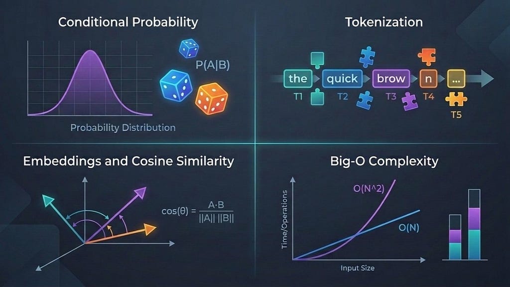
You don’t need to know the math behind why things work the way they do. But it certainly doesn’t hurt. You’ll have a better grasp for what to do when your app gets slow or if your API bill is confusing. In this article, I’ll walk through four key math ideas that will build and sharpen your intuition.
Probability for LLM generation
An LLM doesn’t know answers. It calculates a probability distribution and samples from it.
When you send a prompt to Gemini, it calculates a probability distribution across its vocabulary for the next token. If it’s predicting what follows “The sky is…”, the scores might look like:
- “blue”: 60%
- “clear”: 25%
- “cloudy”: 10%
- “falling”: 3%
- everything else: 2%
The model picks from these weighted options. That’s all generation is: sampling from a probability distribution, repeated thousands of times.
Why the same prompt gives different answers
Run the same prompt twice and you’ll often get two different responses. The probability distribution is the same, but the sampling step introduces genuine randomness. Different tokens get selected each time.
But not all “randomness” is actually from sampling. When you’re vibe coding, your agent is silently building context into every request: the file you’re editing, your open tabs, your cursor position, recent errors. Change any of that and the prompt the model actually sees is different. Different prompt, different probability distribution, different output.
How each word rewrites the odds
Every token the model produces changes the probability distribution for the next one. After picking “blue,” the odds for every possible follow-up shift. “sky” becomes more likely; “banana” drops. This is conditional probability: the chance of the next word given everything so far. Mathematicians write it like this:
P("blue" | "The sky is")
Read the bar | as “given.” This says: what’s the probability of “blue,” given that the prompt so far is “The sky is”? That’s the 60% from the distribution above.
Let’s move on to the next token. Once the model picks “blue,” we start with a new distribution. We are now going to calculate probabilities given “The sky is blue,” which might look like this:
P("and" | "The sky is blue"): 30%
P("today" | "The sky is blue"): 25%
Each token is a new conditional probability, conditioned on everything before it. The full sentence is these probabilities multiplied together, one step at a time — what mathematicians call the chain rule of probability:
P("The sky is blue today") = P("The") × P("sky" | "The") ×
P("is" | "The sky") × P("blue" | "The sky is") ×
P("today" | "The sky is blue")
The takeaway here is that the model isn’t planning a paragraph. It’s making one prediction at a time, and each prediction reshapes the distribution for the next.
What the model pays attention to
Before the model can calculate those conditional probabilities for the next token, it uses a mechanism called attention to decide how much weight each part of your prompt deserves. Think of it as a spotlight for each word it’s about to generate. The model sweeps the spotlight across everything it’s seen and brightens the parts that seem most relevant.
If you ask “What is the capital of France?,” the spotlight focuses on “capital” and “France” while barely glancing at “What” and “is.” That’s why word order and phrasing matter.
Sampling: picking from the distribution
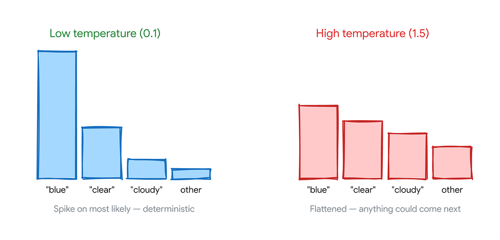
Once the model has its probability distribution for the next token, it has to pick one. That picking process is called sampling, and there are different strategies for it. At one extreme, greedy decoding always picks the single most probable token — deterministic and repeatable, though not perfectly so in practice. At the other extreme, the model samples from the full distribution and lets unlikely tokens have a real shot.
A parameter called temperature controls this tradeoff: lower values sharpen the distribution toward the top token, higher values flatten it out. Another called top-p trims the tail, only sampling among tokens whose probabilities add up to a threshold. In practice, newer models like Gemini 3.5 Flash handle this automatically — Google recommends leaving the defaults alone and letting the model manage its own sampling. You don’t need to tune these parameters. You need to understand that sampling exists.
Token economics
Text gets chopped into tokens, roughly 4 characters each. You pay per token for both your inputs to and the outputs from the model.
Before anything reaches the model, your text is split into tokens by a tokenizer. Gemini uses SentencePiece, which learns subword units from its training corpus. It finds the patterns that appear most often: common words, frequent prefixes and suffixes, and assigns each one a token ID from a fixed vocabulary of size V (typically 32,000–256,000 entries).
“embedding” → [“embed”, “ding”]: 2 tokens
“JavaScript” → [“Java”, “Script”]: 2 tokens
“async” → [“async”]: 1 token (common enough to earn its own ID)
On average, 1 token is roughly 4 characters in English. That length is a consequence of a tradeoff between speed and the size of the vocabulary. If tokens are too short (e.g. single characters), sequences get very long. The model’s attention mechanism gets increasingly more expensive as sequences grow (more details on that in Big-O for scaling). If tokens are too long (e.g. whole words), you’re going to have a long tail of rare vocabulary entries. These entries won’t appear often enough in training to learn anything useful.
Token length will vary based on the domain. For example, code is often cheaper because keywords like function, return, and const are common enough to be single tokens. On the other hand, unique variable names like handleUserAuthCallback would get split into pieces and cost more tokens.
Note that you pay for tokens in both directions, but output tokens cost more. With Gemini 3.5 Flash, input currently runs $1.50 USD per million tokens and output (including thinking tokens) runs $9.00 per million. Output is 6x pricier per token. If you ask the model to “explain in detail,” you’re paying for extra words it generates. To put it in perspective, a standard page of text is around 250 words, which ends up around 300–350 tokens.
Embeddings for semantic search
Common use cases for vibe-coded apps include search and recommendation. Both have a shared foundation in similarity. For search, you may want to return answers that are similar to your question. For recommendation, you’re looking at similar objects to the one your user is browsing. There’s also a Gemini embedding model to support these use cases.
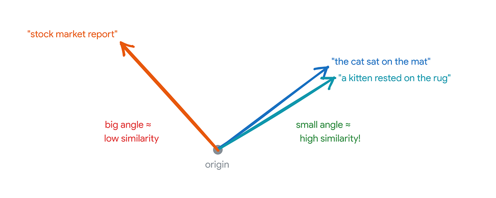
When you send text through an embedding model, it comes back as a list of floating-point numbers. That list is a vector, usually hundreds of dimensions long. You can think of the vector as coordinates that place your text at a specific point in high-dimensional space, or equivalently, as an arrow pointing from the origin to that point.
Let’s say we embed two sentences and get back tiny vectors:
“the cat sat on the mat” → A = [0.8, 0.2]
“a kitten rested on the rug” → B = [0.7, 0.3]
These arrows point in nearly the same direction: both are about felines resting. A third phrase like “stock market report” would produce a vector pointing somewhere else entirely.
Measuring the angle: cosine similarity
To quantify “how similar,” you measure the angle between two vectors using cosine similarity. In the formula below, A · B is the dot product, where you multiply each pair of matching dimensions and add them up. ‖A‖ is the norm, which is the vector’s magnitude, or length. Dividing by both norms cancels out magnitude so you’re left with just the direction:

We can plug in our vectors above to calculate the cosine similarity.

The result is a number between −1 and 1. 0.99 means these two vectors are pointing almost exactly the same way. The model sees them as near-synonyms. A score near 0 means unrelated; near −1 means opposite.
Retrieval-Augmented Generation, or RAG, is just this math at scale. Store your documents as embedding vectors, convert the user’s question to a vector too, compute cosine similarity against every stored vector, and feed the closest matches to the LLM as context. Pro tip: the embedding model you use to store your doc and to convert the user question must match!
Understanding why your app is slow
Let’s picture this scenario. Your app works great on 10 documents. Then you load the real dataset of 100,000 documents, and it crawls. What tools can we use to analyze this situation?
Big-O notation describes the upper bound on how a function grows. When we say an algorithm is O(n²), we mean its running time grows at most proportionally to n² as the input size n increases. It’s a worst-case ceiling, not an exact measurement — your code might be faster in practice, but it won’t be slower than this rate.
Computer scientists have a whole family of these notations: Big-Ω (lower bound — it’s at least this fast), Big-Θ (tight bound — it’s exactly this rate), and little-o (strictly slower than). In everyday coding, Big-O is the one that matters because you’re usually asking: how bad could this get?
The growth rates you’ll see in your code
Here are the common ones, from fast to slow. Don’t worry about memorizing them, you just need to recognize the patterns:
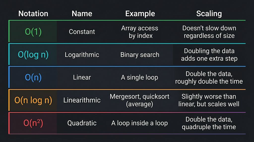
The jump from O(n) to O(n²) is where performance issues become noticeable. Let’s say we have a web app that’s doing a bulk import of users, and it needs to find duplicates. Here’s what the difference in performance between implementations might look like:
// Linear: O(n) - fine at any reasonable size
const names = users.map((u) => u.name);

// Quadratic: O(n²) - fine at 10 users, frozen at 10,000
const duplicates = [];
for (let i = 0; i < users.length; i++) {
  for (let j = i + 1; j < users.length; j++) {
    if (users[i].email === users[j].email) {
      duplicates.push(users[i]);
    }
  }
}
// Fix: use a Set - back to O(n)
const seen = new Set();
const duplicatesFast = users.filter((u) => {
  if (seen.has(u.email)) return true;
  seen.add(u.email);
  return false;
});
That nested loop runs 45 comparisons with 10 users. With 10,000 users, it runs 50 million. Same code, same logic, entirely different performance.
Loops are the most common source of these problems. Any time an O(n) operation like .includes() or an API call runs inside a loop, you might have an O(n²) algorithm. Also, make sure to filter before you sort. Sorting is O(n log n), and there’s no point paying that cost on data you’re about to throw away.
What have we learned here? The gap between a demo and a production app can sometimes be hard to close. Whether you’re a vibe coder or an AI researcher, knowing enough about probability, tokens, embeddings, and complexity helps with asking the right questions. If you want to put these ideas into practice, try Google AI Studio, a web-based prototyping platform, or Antigravity, Google’s agent development platform.
What math concepts do you think are most helpful to the builders of tomorrow? Share with me on X, LinkedIn, or Bluesky.
Four math concepts to improve your vibe coding was originally published in Google Cloud – Community on Medium, where people are continuing the conversation by highlighting and responding to this story.
Source Credit: https://medium.com/google-cloud/four-math-concepts-to-improve-your-vibe-coding-f48ac3964cea?source=rss—-e52cf94d98af—4
About the Author