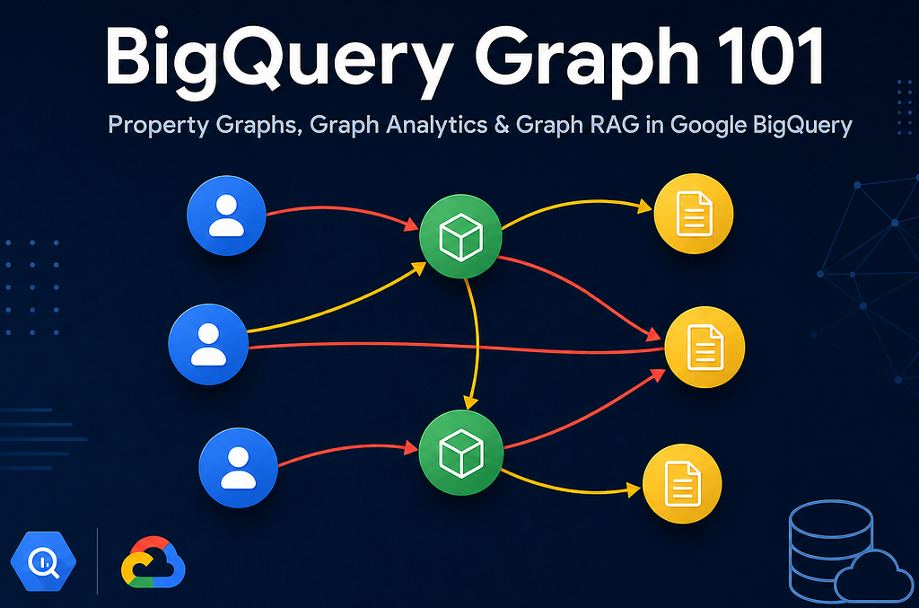
If you have ever worked with data like “customers who bought products” or “users who follow other users,” or “fraud detection” you know that these relationships are intricate and can get messy to query with plain SQL joins. Graph databases were created to make this kind of connected data easier to explore. While there are multiple options for graph databases available in the market, we will explore something which is very native to Google Cloud Platform and is within the data warehouse — BigQuery.
What are Graphs ?
Before we get into BigQuery Graph specifics, let us understand what a “graph database” actually is. A graphdatabase is a database that is optimized for storing and querying highly connected data as nodes (the things, like a Customer or a Product) and relationships (the connections between them, like “PURCHASED” or “VIEWED”) — rather than organizing everything into rows and columns (like a relational database) or nested documents (like a document database).
What are Graph Databases ?
Traditional relational databases can absolutely store connected data, but they start to struggle once your questions require hopping across many relationships. Asking “which customers bought the same product as me?” or “who are my friends-of-friends-of-friends?” usually means chaining together several JOINs — and each additional "hop" in the relationship adds another expensive join, making the query harder to write, harder to read, slower to run, and expensive on compute as the data grows. Graph databases avoids this by storing the relationships as first-class nodes, so "hoping" from one connected thing to another is a fast, natural operation rather than a multi-way JOIN. This node-and-relationship style is often called a property graph model, and it’s the concept behind popular dedicated graph databases like Neo4j, as well as graph query languages such as Cypher and the newer standard GQL.
BigQuery Graph
BigQuery Graphs bring this same property graph model natively into your data warehouse, so you can query connected data without ever exporting it to a separate, specialized graph database. They let you define a graph layer on top of your existing BigQuery tables — no new database, no data duplication, no data movement. You can query them using GQL (Graph Query Language), which is great at answering questions like “what is connected to what.”
With this theory lets do a handson lab. In this blog we will cover —
- A simple retail example with sample data
- Core graph concepts explained simply
- Example queries to traverse the graph
- A small Python example showing how this connects to the idea of “GraphRAG” (Graph Retrieval-Augmented Generation) using LLM
Simple Retail Usecase
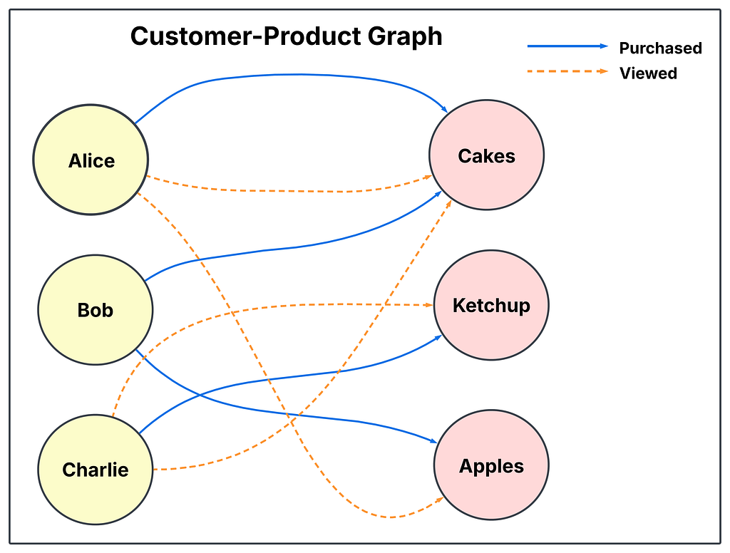
Here’s a quick preview of the graph schema we will build: Customer and Product nodes, connected by PURCHASED and VIEWED edges.
Customer1 (Alice)   --PURCHASED--> Product1 (Cakes)
Customer2 (Bob)     --PURCHASED--> Product1 (Cakes)
Customer2 (Bob)     --PURCHASED--> Product3 (Apple)
Customer3 (Charlie) --PURCHASED--> Product2 (Ketchup)

Customer1 (Alice)   --VIEWED-----> Product3 (Apple)
Customer1 (Alice)   --VIEWED-----> Product1 (Cakes)
Customer3 (Charlie) --VIEWED-----> Product1 (Cakes)
Customer3 (Charlie) --VIEWED-----> Product2 (Ketchup)
Step 1: Create the underlying tables
BigQuery Graphs are built on top of normal BigQuery tables. So first, we will create regular tables.
-- Table of customers (these will become our "Customer" nodes)
CREATE TABLE GCP_PROJECT_ID.DATASET_NAME.customers (
  customer_id STRING NOT NULL,
  name STRING,
  email STRING,
  PRIMARY KEY (customer_id) NOT ENFORCED
);

-- Table of products (these will become our "Product" nodes)
CREATE TABLE GCP_PROJECT_ID.DATASET_NAME.products (
  product_id STRING NOT NULL,
  product_name STRING,
  category STRING,
  price NUMERIC,
  PRIMARY KEY (product_id) NOT ENFORCED
);

-- Table of purchases (these will become our "PURCHASED" edges)
CREATE TABLE GCP_PROJECT_ID.DATASET_NAME.purchases (
  purchase_id STRING NOT NULL,
  customer_id STRING NOT NULL,
  product_id STRING NOT NULL,
  purchase_date DATE,
  PRIMARY KEY (purchase_id) NOT ENFORCED
);

-- Table of views (these will become our "VIEWED" edges)
CREATE TABLE GCP_PROJECT_ID.DATASET_NAME.views (
  view_id STRING NOT NULL,
  customer_id STRING NOT NULL,
  product_id STRING NOT NULL,
  view_date DATE,
  PRIMARY KEY (view_id) NOT ENFORCED
);
Step 2: Insert some sample data
Let us add the sample retail data as discussed in our usecase.
-- Sample customers
INSERT INTO GCP_PROJECT_ID.DATASET_NAME.customers (customer_id, name, email) VALUES
  ('C1', 'Alice',   'alice@example.com'),
  ('C2', 'Bob',     'bob@example.com'),
  ('C3', 'Charlie', 'charlie@example.com');

-- Sample products
INSERT INTO GCP_PROJECT_ID.DATASET_NAME.products (product_id, product_name, category, price) VALUES
  ('P1', 'Cakes',   'Bakery',     12.99),
  ('P2', 'Ketchup', 'Condiments',  4.99),
  ('P3', 'Apple',   'Produce',     0.99);

-- Sample purchases
INSERT INTO GCP_PROJECT_ID.DATASET_NAME.purchases (purchase_id, customer_id, product_id, purchase_date) VALUES
  ('PU1', 'C1', 'P1', '2026-01-05'),
  ('PU2', 'C2', 'P1', '2026-01-10'),
  ('PU3', 'C2', 'P3', '2026-02-01'),
  ('PU4', 'C3', 'P2', '2026-02-15');

-- Sample views (a customer looked at a product, may or may not have purchased it)
INSERT INTO GCP_PROJECT_ID.DATASET_NAME.views (view_id, customer_id, product_id, view_date) VALUES
  ('V1', 'C1', 'P3', '2026-01-01'),
  ('V2', 'C1', 'P1', '2026-01-04'),
  ('V3', 'C3', 'P1', '2026-02-10'),
  ('V4', 'C3', 'P2', '2026-02-14');
Step 3: Create the property graph
One of the crucial steps. Wiring these tables together into a graph using CREATE PROPERTY GRAPH.
CREATE OR REPLACE PROPERTY GRAPH `PROJECT_ID.DATASET_NAME.retail_graph`
  NODE TABLES (
    `PROJECT_ID.DATASET_NAME.customers` AS Customer
      KEY (customer_id)
      LABEL Customer
      PROPERTIES (customer_id, name, email),

    `PROJECT_ID.DATASET_NAME.products` AS Product
      KEY (product_id)
      LABEL Product
      PROPERTIES (product_id, product_name, category, price)
  )
  EDGE TABLES (
    `PROJECT_ID.DATASET_NAME.purchases`
      KEY (purchase_id)
      SOURCE KEY (customer_id) REFERENCES Customer (customer_id)
      DESTINATION KEY (product_id) REFERENCES Product (product_id)
      LABEL PURCHASED
      PROPERTIES (purchase_date),

    `PROJECT_ID.DATASET_NAME.views`
      KEY (view_id)
      SOURCE KEY (customer_id) REFERENCES Customer (customer_id)
      DESTINATION KEY (product_id) REFERENCES Product (product_id)
      LABEL VIEWED
      PROPERTIES (view_date)
  );
Output:
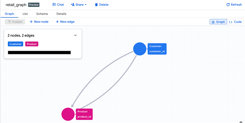
We now have a graph called retail_graph sitting on top of our four regular tables. No data was copied or moved — BigQuery just knows how to interpret these tables as a connected graph when we query it that way.
Core Graph Terminologies:
Before moving further, let us get our concepts cleared.
- Node — A single “thing” or “entity” in your data. In our example, a Customer or a Product is a node.
- Edge — A connection or relationship between two nodes. In our example, PURCHASED and VIEWED are edges — they're the lines connecting a Customer circle to a Product circle. Edges usually have a direction (Customer → Product), showing who did what to whom.
- Property — An attribute or piece of information attached to a node or edge. For example, a Customer node has properties like name and email. A PURCHASED edge has a property like purchase_date. Properties are like the extra details of the node.
- Label — A category name for a node or edge, used to group similar things. All customer rows get the label Customer; all purchase rows get the label PURCHASED. Labels let you say "find all Customer nodes" instead of listing every one individually — like a folder name for similar items.
- Key — The unique identifier for a node or edge (similar to a primary key in a normal table). It’s how BigQuery knows which row is which node, and how edges know which nodes they connect to.
- Property Graph — This is the overall concept: a logical view that layers nodes, edges, labels, and properties on top of your existing relational tables.
Example 1: What did a customer purchase? (1-hop query)
BigQuery lets you query graphs using GQL (Graph Query Language) through a special function called GRAPH_TABLE. Instead of writing joins, you write MATCH patterns that look like little diagrams of what you want to find — arrows and all.
SELECT *
FROM GRAPH_TABLE(
  `PROJECT_ID.DATASET_NAME.retail_graph`,
  MATCH (c:Customer)-[purchased:PURCHASED]->(p:Product)
  WHERE c.name = 'Alice'
  RETURN c.name AS customer_name,
         p.product_name AS product_name,
         purchased.purchase_date AS purchase_date
) AS t;
Output:

This is the simplest kind of graph query — just one connection (“hop”) away. This reads as: “Find Customer nodes connected by a PURCHASED edge to a Product node, filter to Alice, and return the customer’s name, the product’s name, and when it was purchased.”
Example 2: Products viewed and then purchased (a slightly richer pattern)
Let’s find cases where a customer viewed a product and also purchased that same product — useful for understanding “search then buy” behavior in retail.
SELECT *
FROM GRAPH_TABLE(
  `PROJECT_ID.DATASET.retail_graph`,
  MATCH (c:Customer)-[v:VIEWED]->(p:Product),
        (c)-[pu:PURCHASED]->(p)
  RETURN c.name AS customer_name,
         p.product_name AS product_name,
         v.view_date AS viewed_on,
         pu.purchase_date AS purchased_on
) AS t;
Output:

Here we reused the same customer c and product p in two patterns, telling GQL: "the customer who viewed this product is the same customer who purchased it, and it's the same product both times."
Example 3: Customers who purchased the same product as another customer (2-hop traversal)
This is a great example of graph traversal being much easier to read than the equivalent SQL self-join. We want to find pairs of different customers who bought the same product — useful for “customers like you also bought” style recommendations.
SELECT *
FROM GRAPH_TABLE(
  `PROJECT_ID.DATASET_NAME.retail_graph`
  MATCH (c1:Customer)-[:PURCHASED]->(p:Product)<-[:PURCHASED]-(c2:Customer)
  WHERE c1.customer_id < c2.customer_id
  RETURN c1.name AS customer_1,
         c2.name AS customer_2,
         p.product_name AS shared_product
) AS t;
Output:

Here, the pattern (c1)-[:PURCHASED]->(p)<-[:PURCHASED]-(c2): it walks from customer 1, to the product, and then backwards from customer 2. This is a 2-hop traversal (Customer → Product → Customer), and it's the kind of query that graph query languages make especially readable compared to writing multiple joins by hand.
A Simple GraphRAG Python Example using LLM
Now let’s connect this using: GraphRAG, short for Graph Retrieval-Augmented Generation. The core idea of RAG (Retrieval-Augmented Generation) is instead of asking an LLM (Large Language Model) a question with no context, you first retrieve relevant facts from your own data, and then feed those facts to the LLM as context so it can give a grounded, accurate answer. GraphRAG simply means the “retrieval” part comes from a graph — pulling out connected, relevant information (like a customer’s purchases and related products) rather than just plain keyword search.
Usecase:
We will retrieves a customer’s purchase/view history by traversing a BigQuery property graph (Customer → Product relationships). We will feed that graph-derived context into an LLM as a grounding and then geenrate a personalized, explainable product recommendation for that customer based only on their actual graph history. I have used simple GitHub Marketplace model — openai/gpt-4o.
Code:
import os
from google.cloud import bigquery
from openai import OpenAI


PROJECT_ID = os.environ.get("PROJECT_ID", "your-gcp-project-id")
DATASET = os.environ.get("DATASET", "dataset_name")
GRAPH_NAME = os.environ.get("GRAPH_NAME", "retail_graph")
GITHUB_MODELS_BASE_URL = "https://models.github.ai/inference"
MODEL_NAME = os.environ.get("MODEL_NAME", "openai/gpt-4o")

client = bigquery.Client(project=PROJECT_ID)

# Step 1: Retrieval -- pull a customer's purchase/view subgraph from BigQuery

def get_customer_graph_context(customer_name: str) -> list:
    """
    Run a GQL query against the BigQuery property graph to retrieve a
    customer's purchased and viewed products.

    Returns a list of dicts, each describing one relationship, e.g.:
        [
            {"relationship": "PURCHASED", "product_name": "Cakes", "category": "Bakery"},
            {"relationship": "VIEWED", "product_name": "Apple", "category": "Produce"},
            ...
        ]
    """

    query = f"""
    SELECT relationship, product_name, category
    FROM GRAPH_TABLE(
      `{PROJECT_ID}.{DATASET}.{GRAPH_NAME}`
      MATCH (c:Customer)-[e:PURCHASED|VIEWED]->(p:Product)
      WHERE c.name = @customer_name
      RETURN LABELS(e)[OFFSET(0)] AS relationship,
            p.product_name AS product_name,
            p.category AS category
    ) AS t
    """

    job_config = bigquery.QueryJobConfig(
        query_parameters=[
            bigquery.ScalarQueryParameter("customer_name", "STRING", customer_name)
        ]
    )

    rows = client.query(query, job_config=job_config).result()

    context = []
    for row in rows:
        context.append(
            {
                "relationship": row.relationship,
                "product_name": row.product_name,
                "category": row.category,
            }
        )

    return context

# Step 2: Context formatting -- turn graph rows into natural-language text

def format_context_as_text(customer_name: str, graph_context: list) -> str:
    """
    Convert structured graph query results into a natural-language context
    string suitable for prompting an LLM, e.g.:

        "Alice purchased: Cakes. Alice viewed: Apple, Cakes."
    """

    purchased = [row["product_name"] for row in graph_context if row["relationship"] == "PURCHASED"]
    viewed = [row["product_name"] for row in graph_context if row["relationship"] == "VIEWED"]

    parts = []

    if purchased:
        parts.append(f"{customer_name} purchased: {', '.join(purchased)}.")
    else:
        parts.append(f"{customer_name} has no recorded purchases.")

    if viewed:
        parts.append(f"{customer_name} viewed: {', '.join(viewed)}.")
    else:
        parts.append(f"{customer_name} has no recorded views.")

    return " ".join(parts)


# Step 3: Generation -- call GitHub Models (OpenAI-compatible API) for a
# grounded recommendation based on the retrieved graph context

def ask_github_models(context_text: str) -> str:
    """
    Send the graph-derived context plus a recommendation question to
    GitHub Models' inference API (OpenAI-compatible SDK), and return the
    model's text response.
    """

    github_token = os.environ.get("GITHUB_TOKEN")
    if not github_token:
        raise RuntimeError(
            "GITHUB_TOKEN environment variable is not set. "
            "Run: export GITHUB_TOKEN=xxxxxxxxxxxxxxxx"
        )

    llm_client = OpenAI(
        base_url=GITHUB_MODELS_BASE_URL,
        api_key=github_token,
    )

    system_prompt = (
        "You are a helpful retail recommendation assistant. You are given "
        "a customer's purchase and viewing history, retrieved from a "
        "product/customer graph. Use only this context to make a specific, "
        "well-reasoned product recommendation."
    )

    user_prompt = (
        f"Customer graph context:\n{context_text}\n\n"
        "What should we recommend to this customer next, and why, based on "
        "their purchase/view graph?"
    )

    response = llm_client.chat.completions.create(
        model=MODEL_NAME,
        messages=[
            {"role": "system", "content": system_prompt},
            {"role": "user", "content": user_prompt},
        ],
    )

    return response.choices[0].message.content


def main():
    customer_name = "Alice"

    # Step 1: Retrieve graph context from BigQuery
    graph_context = get_customer_graph_context(customer_name)

    # Step 2: Format the graph context as natural-language text
    context_text = format_context_as_text(customer_name, graph_context)
    print("----- Graph context -----")
    print(context_text)
    print("--------------------------")

    recommendation = ask_github_models(context_text)

    print("----- LLM recommendation -----")
    print(recommendation)
    print("-------------------------------")


if __name__ == "__main__":
    main()
Output:
----- Graph context -----
Alice purchased: Cakes. Alice viewed: Apple, Cakes.
--------------------------
----- LLM recommendation -----
Based on Alice's purchase and viewing history, I recommend suggesting Apples next. Here's why:

- Alice has already purchased Cakes, which indicates an interest in sweet and food-related products.
- She has viewed both Cakes and Apples, showing some level of curiosity about Apples in particular.
- Since she hasn’t purchased Apples yet, recommending them aligns with her browsing behavior and could lead to a conversion.

This recommendation caters to her demonstrated interest in food and her specific engagement with Apples.
-------------------------------
Conclusion
BigQuery Graphs give you a way to model and query connected and relationships bewteen them without leaving BigQuery or standing up a separate graph database. You define nodes and edges on top of your existing tables using CREATE PROPERTY GRAPH, and then use GQL's intuitive MATCH patterns to traverse relationships that would otherwise require complex, hard-to-read joins. In this blog, we walked through the full loop — creating tables, defining a small retail property graph, understanding the core vocabulary (nodes, edges, properties, labels, keys), running increasingly rich traversal queries, and finally sketching out how this graph can power a simple GraphRAG pipeline to give an LLM real, grounded context. If you’re already using BigQuery, graphs are a low-friction way to start thinking in terms of relationships — simple and no migration required. Thats it from this blog of mine, suggestions are most welcomed.
BigQuery Graphs 101: A Retail usecase with GQL and GraphRAG was originally published in Google Cloud – Community on Medium, where people are continuing the conversation by highlighting and responding to this story.
Source Credit: https://medium.com/google-cloud/bigquery-graphs-101-a-retail-usecase-with-gql-and-graphrag-92641e35ef6b?source=rss—-e52cf94d98af—4
About the Author